Visualizing results

This notebook shows how to run simulations with different algorithms, collect results, and visualize them on several plots to compare the algorithms’ performances.

Setup environment

First, we create the environment in which the simulations will take place. We simply use the “basic” (default) environment, to simplify. Because this document is executed in the docs/ folder, we need to change the current working directory to import the data files correctly; on a typical setup, only the following lines are necessary:

from smartgrid import make_basic_smartgrid
from algorithms.qsom import QSOM
from algorithms.naive import RandomModel

env = make_basic_smartgrid()

We will execute simulations for 50 time steps, to limit the required time to render this notebook and build the documentation. Typically, 10,000 time steps are used for a simulation, taking about ~ 1 or 2 hours, depending on the machine. Simulations with 100 or 1,000 time steps can be a nice compromise between number of data points and execution time.

We also set the seed to some pre-defined constant, to ensure reproducibility of results.

max_step = 50
seed = 1234

Run simulations and collect results

Now, we run a simulation using a first algorithm, QSOM. This algorithm is already provided in this project, so using it is straightforward.

We collect rewards received by learning agents at each time step in an array for visualizing later. To simplify the plotting process, we will only memorize the average of rewards at each time step; more complex plots can be created by logging more details, such as all rewards received by all learning agents at each time step.

import numpy as np

data_qsom = []
model_qsom = QSOM(env)

obs = env.reset(seed=seed)
for step in range(max_step):
    actions = model_qsom.forward(obs)
    obs, rewards, _, _, _ = env.step(actions)
    model_qsom.backward(obs, rewards)
    # Memorize the average of rewards received at this time step
    data_qsom.append(np.mean(rewards))

/home/runner/.local/lib/python3.10/site-packages/gymnasium/core.py:311: UserWarning: WARN: env.n_agent to get variables from other wrappers is deprecated and will be removed in v1.0, to get this variable you can do `env.unwrapped.n_agent` for environment variables or `env.get_wrapper_attr('n_agent')` that will search the reminding wrappers.
  logger.warn(

To compare QSOM with another algorithm, we will run a simulation with a Random model, taking actions completely randomly. This algorithm is also already provided in this project, allowing us to focus on running simulations and plotting results here. For more interesting comparisons, other learning algorithms should be implemented, or re-used from existing projects, such as Stable Baselines.

data_random = []
model_random = RandomModel(env, {})

obs = env.reset(seed=seed)
for step in range(max_step):
    actions = model_random.forward(obs)
    obs, rewards, _, _, _ = env.step(actions)
    model_random.backward(obs, rewards)
    # Memorize the average of rewards received at this time step
    data_random.append(np.mean(rewards))

Plot results

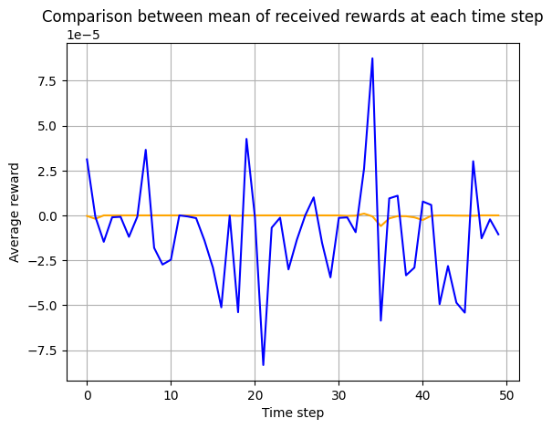
We now have the results (average of rewards per time step) for two simulations using two different algorithms. We can visualize them using a plotting library; to keep it simple, we will use Matplotlib here, but any library can be used, such as seaborn, bokeh, …

import matplotlib.pyplot as plt

x = list(range(max_step))
plt.plot(x, data_qsom, color='orange', label='QSOM')
plt.plot(x, data_random, color='blue', label='Random')
plt.grid()
plt.xlabel('Time step')
plt.ylabel('Average reward')
plt.title('Comparison between mean of received rewards at each time step')
plt.show()

Note that, with only a few time steps, it is difficult to compare these algorithms. We emphasize again that, in most cases, simulations should run for many more steps, e.g., 10,000.

Other plots can be created, e.g., collecting all agents’ rewards and showing the confidence interval of them per time step; running several simulations and plotting the distribution of scores, i.e., average of average rewards per learning agent per time step, etc.